Example 9.37: (Mis)behavior of binomial confidence intervals

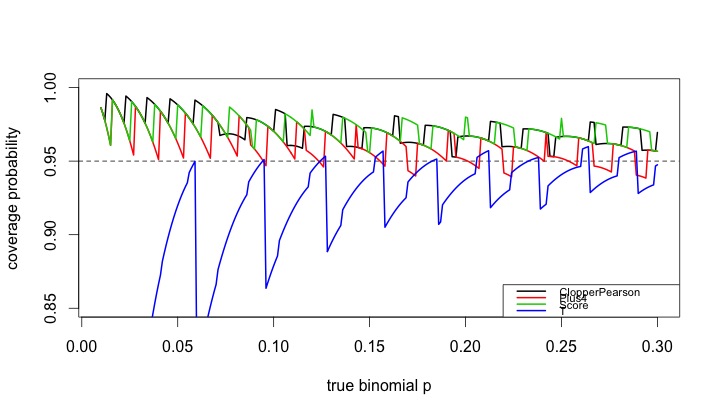
While traditional statistics courses teach students to calculate intervals and test for binomial proportions using a normal or t approximation, this method does not always work well. Agresti and Coull ("Approximate is better than "exact' for interval estimation of binomial proportions". The American Statistician, 1998; 52:119-126) demonstrated this and reintroduced an improved (Plus4) estimator originally due to Wilson (1927).

In this entry, we demonstrate how the coverage varies as a function of the underlying probability and compare four intervals: (1) t interval, (2) Clopper-Pearson, (3) Plus4 (Wilson/Agresti/Coull) and (4) Score, using code contributed by Albyn Jones from Reed College. Here, coverage probability is defined as the expected value that a CI based on an observed value will cover the true binomial parameter that generated that value. The code calculates the coverage probability as a function of a given binomial probability p and a sample size n. Intervals are created for each of the possible outcomes from 0, ..., n, then checked to see if the intervals include the true value. Finally, the sum of the probabilities of observing outcomes in which the binomial parameter is included in the interval determines the exact coverage. Note several distinct probabilities: (1) binomial parameter "p", the probability of success on a trial; (2) probability of observing x successes in N trials, P(X=x); (3) coverage probability as defined above. For distribution quantiles and probabilities, see section 1.10 and table 1.1.

R

We begin by defining the support functions which will be used to calculate the coverage probabilities for a specific probability and sample size.

CICoverage = function(n, p, alpha=.05) {
  # set up a table to hold the results
  Cover = matrix(0, nrow=n+1, ncol=5)
  colnames(Cover)=c("X","ClopperPearson","Plus4","Score","T")
  Cover[,1]=0:n
  zq = qnorm(1-alpha/2)
  tq = qt(1-alpha/2,n-1)
  for (i in 0:n) {
    Phat = i/n
    P4 = (i+2)/(n+4)
    # Calculate T and plus4 intervals manually, 
    # use canned functions for the other 
    TInt = Phat + c(-1,1)*tq*sqrt(Phat*(1-Phat)/n)
    P4Int = P4 + c(-1,1)*zq*sqrt(P4*(1-P4)/(n+4))
    CPInt= binom.test(i,n)$conf.int
    SInt = prop.test(i,n)$conf.int
    # check to see if the binomial p is in each CI 
    Cover[i+1,2] = InInt(p, CPInt)
    Cover[i+1,3] = InInt(p, P4Int)
    Cover[i+1,4] = InInt(p, SInt)
    Cover[i+1,5] = InInt(p, TInt)
  }
  # probability that X=x 
  p = dbinom(0:n, n, p)
  ProbCover=rep(0, 4)
  names(ProbCover) = c("ClopperPearson", "Plus4", "Score", "T")
  # sum P(X=x) * I(p in CI from x)
  for (i in 1:4){
    ProbCover[i] = sum(p*Cover[,i+1])
  }
  list(n=n, p=p, Cover=Cover, PC=ProbCover)
}

In addition, we define a function to determine whether something is in the interval.

InInt = function(p,interval){
  interval[1] <= p && interval[2] >= p
}

Finally, there's a function which summarizes the results.

CISummary = function(n, p) {
  M = matrix(0,nrow=length(n)*length(p),ncol=6)
  colnames(M) = c("n","p","ClopperPearson","Plus4","Score","T")
  k=0
  for (N in n) {
    for (P in p) {
      k=k+1
      M[k,]=c(N, P, CICoverage(N, P)$PC)
    }
  }
  data.frame(M)
}

We then generate the CI coverage plot provided at the start of the entry, which uses sample size n=50 across a variety of probabilities.

lwdval = 2
nvals = 50
probvals = seq(.01, .30, by=.001)
results = CISummary(nvals, probvals)
plot(range(probvals), c(0.85, 1), type="n", xlab="true binomial p",
     ylab="coverage probability")
abline(h=0.95, lty=2)
lines(results$p, results$ClopperPearson, col=1, lwd=lwdval)
lines(results$p, results$Plus4, col=2, lwd=lwdval)
lines(results$p, results$Score, col=3, lwd=lwdval)
lines(results$p, results$T, col=4, lwd=lwdval)
tests = c("ClopperPearson", "Plus4", "Score", "T")
legend("bottomright", legend=tests,
       col=1:4, lwd=lwdval, cex=0.70)

The resulting plot is quite interesting, and demonstrates how non-linear the coverage is for these methods, and how the t (almost equivalent to the normal, in this case) is anti-conservative in many cases. It also confirms the results of Agresti and Coull, who concluded that for interval estimation of a proportion, coverage probabilities from inverting the standard binomial and too small when inverting the Wald large-sample normal test, with the Plus 4 yielding coverage probabilities close to the desired, even for very small sample sizes.

SAS
Calculating the coverage probability for a given N and binomial p can be done in a single data step, summing the probability-weighted coverage indicators over the realized values of the random variate. Once this machinery is developed, we can call it repeatedly, using a macro, to find the results for different binomial p. We comment on the code internally.

%macro onep(n=,p=,alpha=.05);
data onep;
n = &n;
p = &p;
alpha = α
/* set up collectors of the weighted coverage indicators */
expcontrib_t = 0;
expcontrib_p4 = 0;
expcontrib_s = 0;
expcontrib_cp = 0;
/* loop through the possible observed successes x*/
do x = 0 to n;
  probobs = pdf('BINOM',x,p,n);  /* probability X=x */
  phat = x/n;
  zquant = quantile('NORMAl', 1 - alpha/2, 0, 1);
  p4 = (x+2)/(n + 4);

  /* calculate the half-width of the t and plus4 intervals */
  thalf = quantile('T', 1 - alpha/2,(n-1)) * sqrt(phat*(1-phat)/n);
  p4half = zquant * sqrt(p4*(1-p4)/(n+4));

  /* the score CI in R uses a Yates correction by default, and is 
     reproduced here */
  yates = min(0.5, abs(x - (n*p)));
  z22n = (zquant**2)/(2*n);
  yl = phat-yates/n;
  yu = phat+yates/n;
  slower = (yl + z22n - zquant * sqrt( (yl*(1-yl)/n) + z22n / (2*n) )) /
    (1 + 2 * z22n); 
  supper = (yu + z22n + zquant * sqrt( (yu*(1-yu)/n) + z22n / (2*n) )) /
    (1 + 2 * z22n); 

  /* cover = 1 if in the CI, 0 else */
  cover_t = ((phat - thalf) < p) and ((phat + thalf) > p);
  cover_p4 = ((p4 - p4half) < p) and ((p4 + p4half) > p);
  cover_s = (slower < p) and (supper > p);
  /* the Clopper-Pearson interval can be easily calculated on the fly */ 
  cover_cp = (quantile('BETA', alpha/2 ,x,n-x+1) < p) and 
    (quantile('BETA', 1 - alpha/2 ,x+1,n-x) > p); 

  /* cumulate the weighted probabilities */
  expcontrib_t = expcontrib_t + probobs * cover_t;
  expcontrib_p4 = expcontrib_p4 + probobs * cover_p4;
  expcontrib_s = expcontrib_s + probobs * cover_s;
  expcontrib_cp = expcontrib_cp + probobs * cover_cp;
  /* only save the last interation */
  if x = N then output;
  end;
run;
%mend onep;

The following macro calls the first one for a series of binomial p for a fixed N. Since the macro %do loop can only iterate through integers, we have to do a little division; the %sysevelf function will do this within the macro.

%macro repcicov(n=, lop=, hip=, byp=, alpha= .05);
/* need an empty data set to store the results */
data summ; set _null_; run;
%do stepp = %sysevalf(&lop / &byp, floor) %to %sysevalf(&hip / &byp,floor);
  /* note that the p sent to the %onep macro is a 
                           text string like "49 * .001" */
  %onep(n = &n, p = &stepp * &byp, alpha = &alpha);
  /* tack on the current results to the ones finished so far */
  /* this is a simple but inefficient way to add each binomial p into 
     the output data set */
  data summ; set summ onep; run;
%end;
%mend repcicov;

/* same parameters as in R */
%repcicov(n=50, lop = .01, hip = .3, byp = .001);

Finally, we can plot the results. One option shown here and not mentioned in the book are the mode=include option to the symbol statement, which allows the two distinct pieces of the T coverage to display correctly.

goptions reset=all;
legend1 label=none position=(bottom right inside)
        mode=share across=1 frame value = (h=2);
axis1 order = (0.85 to 1 by 0.05) minor=none 
   label = (a=90 h=2 "Coverage probability") value=(h=2);
axis2 order = (0 to 0.3 by 0.05) minor=none 
   label = (h=2 "True binomial p") value=(h=2);
symbol1 i = j v = none l =1 w=3 c=blue mode=include;
symbol2 i = j v = none l =1 w=3 c=red;
symbol3 i = j v = none l =1 w=3 c=lightgreen;
symbol4 i = j v = none l =1 w=3 c=black;
proc gplot data = summ;
plot (expcontrib_t expcontrib_p4  expcontrib_s  expcontrib_cp) * p 
  / overlay legend vaxis = axis1 haxis = axis2 vref = 0.95 legend = legend1;
label expcontrib_t = "T approximation" expcontrib_p4 = "P4 method"
      expcontrib_s = "Score method" expcontrib_cp = "Exact (CP)";
run; quit;

An unrelated note about aggregators:We love aggregators! Aggregators collect blogs that have similar coverage for the convenience of readers, and for blog authors they offer a way to reach new audiences. SAS and R is aggregated by R-bloggers, PROC-X, and statsblogs with our permission, and by at least 2 other aggregating services which have never contacted us. If you read this on an aggregator that does not credit the blogs it incorporates, please come visit us at SAS and R. We answer comments there and offer direct subscriptions if you like our content. In addition, no one is allowed to profit by this work under our license; if you see advertisements on this page, the aggregator is violating the terms by which we publish our work.

Example 8.34: lack of robustness of t test with small n

Tim Hesterberg has effectively argued for a larger role for resampling based inference in introductory statistics courses (and statistical practice more generally). While the Central Limit Theorem is a glorious result, and the Student t-test remarkably robust, there are subtleties that Hesterberg, Jones and others have pointed out that are not always well understood.

In this entry, we explore the robustness of the Student one sample t-test in terms of coverage probabilities where we look whether the alpha level is split evenly between the two tails.

R
We begin by defining a function to carry out the simulation study.

runsim = function(FUNCTION=rnorm, n=20, numsim=100000, 
    label="normal") 
{
  missupper = numeric(numsim)
  misslower = numeric(numsim)
  for (i in 1:numsim) {
    x = FUNCTION(n)
    testval = t.test(x)
    missupper[i] = testval$conf.int[2] < 0
    misslower[i] = testval$conf.int[1] > 0
  }
  cat("n=", n,", number of simulations=", numsim, sep="")
  cat(", (true data are ", label, ")\n", sep="")
  cat(round(100*sum(missupper)/numsim, 1), 
    "% of simulations had CI below the true value.\n", sep="")
  cat(round(100*sum(misslower)/numsim, 1), 
    "% of simulations had CI above the true value.\n", sep="")
}

We can define three functions to explore: one where the data are actually normally distributed (so the central limit theorem doesn't need to be invoked), a symmetric distribution (where the central limit theorem can be used with smaller sample sizes) and a skewed distribution (where the central limit theorem requires very large sample sizes).

reallynormal = function(n) { return(rnorm(n)) }
symmetric = function(n) { return(runif(n, -1, 1)) }
skewed = function(n) { return(rexp(n, 1) - 1) }

The results (at least to us) are somewhat startling. To get the tail probabilities correct when the underlying distribution is actually skewed, we need a huge sample size:

> runsim(reallynormal, n=20, label="normal")
n=20, number of simulations=1e+05, (true data are normal)
2.5% of simulations had CI below the true value.
2.5% of simulations had CI above the true value.

> runsim(symmetric, n=20, label="symmetric")
n=20, number of simulations=1e+05, (true data are symmetric)
2.6% of simulations had CI below the true value.
2.5% of simulations had CI above the true value.

> runsim(skewed, n=20, label="skewed")
n=20, number of simulations=1e+05, (true data are skewed)
7.7% of simulations had CI below the true value.
0.6% of simulations had CI above the true value.

> runsim(skewed, n=100, label="skewed")
n=100, number of simulations=1e+05, (true data are skewed)
4.5% of simulations had CI below the true value.
1.2% of simulations had CI above the true value.

> runsim(skewed, n=500, label="skewed")
n=500, number of simulations=1e+05, (true data are skewed)
3.4% of simulations had CI below the true value.
1.7% of simulations had CI above the true value.

SAS

In the SAS version, we'll write a macro that first generates all of the data, then uses by processing to perform the t tests, and finally tallies the results and prints them to the output.

%macro simt(n=20, numsim=100000, myrand=normal(0), label=normal);
data test;
do sim = 1 to &numsim;
  do i = 1 to &n;
    x = &myrand;
    output;
  end;
end;
run;

ods select none;
ods output conflimits=ttestcl;
proc ttest data=test;
  by sim;
  var x;
run;
ods select all;

data _null_;
set ttestcl end=last;
retain missupper 0 misslower 0;
missupper = missupper + (upperclmean lt 0);
misslower = misslower + (lowerclmean gt 0);
if last then do;
  missupper_pct = compress(round(100 * missupper/&numsim,.1));
  misslower_pct = compress(round(100 * misslower/&numsim,.1));
  file print;
  put "n=&n, number of simulations = &numsim, true data are &label"; 
  put missupper_pct +(-1) "% of simulations had CI below the true value";
  put misslower_pct +(-1) "% of simulations had CI above the true value";
end;
run;
%mend simt;

Two or three features of this code bear commenting. First, the retain statement and end option allow us to count the number of misses without an additional data step and/or procedure. Next, the file print statement redirects the results from a put statement to the output, rather than the log. While this is not really needed, the output is where we expect the results to appear. Finally, the odd +(-1) in the final two put statements moves the column pointer back one space. This allows the percent sign to immediately follow the number.

The various distributions and sample sizes used in the R code can be called as follows:

%simt(numsim=100000, n = 20, myrand = normal(0));
%simt(numsim=100000, n = 20, myrand = (2 * uniform(0)) - 1, label=symmetric);
%simt(numsim=100000, n = 20, myrand = (ranexp(0) - 1), label=skewed);
%simt(numsim=100000, n = 100, myrand = (ranexp(0) - 1), label=skewed);
%simt(numsim=100000, n = 500, myrand = (ranexp(0) - 1), label=skewed);

where the code to generate the desired data is passed to the macro as a character string. The results of
%simt(numsim=100000, n = 100, myrand = (ranexp(0) - 1), label=skewed);
are

n=100, number of simulations = 100000, true data are skewed
4.5% of simulations had CI below the true value
1.2% of simulations had CI above the true value

which agrees nicely with the R results above.

We look forward to Tim's talk at the JSM.