Really useful R package: sas7bdat

For SAS users, one hassle in trying things in R, let alone migrating, is the difficulty of getting data out of SAS and into R. In our book (section 1.2.2) and in a blog entry we've covered getting data out of SAS native data sets. Unfortunately, for all of these methods, you need a working, licensed version of SAS.

However Matt Shotwell has reverse-engineered the sas7bdat file format. This means that you can now read a SAS data set without a working copy of SAS. This is a wonderful thing, and in fact SAS Institute ought to have provided this ability long ago. The package is experimental, but it worked fine for two small data sets. Matt tells me that as of 7/2011, the package only works for sas7bdat files generated on 32-bit Windows systems.

R
Install the package sas7bdat. The use the read.sas7bdat() function.

library(sas7bdat)
helpfromSAS = read.sas7bdat("http://www.math.smith.edu
/sasr/datasets/help.sas7bdat")

(Note that newlines are not allowed in the URL in practice, but formatting for the blog required it.)

> is.data.frame(helpfromSAS)
[1] TRUE
> summary(helpfromSAS$MCS)
   Min. 1st Qu.  Median    Mean 3rd Qu.    Max. 
  6.763  21.680  28.600  31.680  40.940  62.180 
> with(helpfromSAS, summary(SUBSTANCE))
alcohol cocaine  heroin 
    177     152     124

It's unclear why all the variable names are all capitalized. That didn't happen in another trial, so it must be something about the way the help.sas7bdat data set was constructed.

Example 7.9: Get data from SAS into R

Some people use both SAS and R in their daily work. They might be more familiar with SAS as a tool for manipulating data and R preferable for plotting purposes. While our goal in the book is to enable people to avoid having to switch back and forth, the following example shows how to move data from SAS into R. Our use of Stata format as an interchange mechanism is perhaps unorthodox, but eminently workable. Other file formats (see section 1.2.2, creating files for use by other packages) can also be specified.

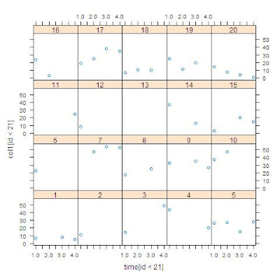
Suppose we wanted to plot CESD over time for each individual. While we show how to do this sort of thing in SAS (see section 5.6.2), it’s hard to do without SAS version 9.2. Instead, we recall it’s easy using the lattice library in R (see section 5.2.2). But we need a ”long” data set with a row for each time point. This is the sort of data management one might prefer to do in SAS.

SAS

First, we read the data from a data set stored in SAS format. Then we use proc transpose (section 1.5.3) to get the data into the required shape. Finally, we save the ”long” data set in Stata format (1.2.2).

libname k "c:\book";

proc transpose data=k.help out=ds1;
by id;
var cesd1 cesd2 cesd3 cesd4;
run;

proc print data = ds1 (obs = 5); run;

 Obs    ID    _NAME_    _LABEL_    COL1

   1     1    CESD1     1 cesd       7 
   2     1    CESD2     2 cesd       . 
   3     1    CESD3     3 cesd       8 
   4     1    CESD4     4 cesd       5 
   5     2    CESD1     1 cesd      11 


proc export data=ds1 (rename=(_label_=timec1))
   outfile = "c:\book\helpfromsas.dta" dbms=dta;
run;

R
In R, we first read the file from Stata format (1.1.5), then attach() it (section 1.3.1) for ease of typing. Then we check the first few lines of data using the head() function (section 1.13.1). Noting that the time variable we brought from SAS is a character string, we convert it to a numeric variable using as.numeric() (section 1.4.2) and substr() (section 1.4.3). After loading the lattice library, we display the series for each subject. In this, we use the syntax for subsetting observations (1.5.1) to keep only the first 20 observations and the as.factor() function (1.4.10) to improve the labels in the output.

> library(foreign)
> xsas <- read.dta("C:\\book\\helpfromsas.dta")
> head(xsas)

  id _name_ timec1 col1
1  1  CESD1 1 cesd    7
2  1  CESD2 2 cesd   NA
3  1  CESD3 3 cesd    8
4  1  CESD4 4 cesd    5
5  2  CESD1 1 cesd   11
6  2  CESD2 2 cesd   NA

> attach(xsas)
> time <- as.numeric(substr(timec1, 1, 1))
> library(lattice)
> xyplot(col1[id < 21] ~ time[id < 21]|as.factor(id[id < 21]))

In the next entry, we'll reverse this process to manipulate data in R and produce the plot in SAS.