SAS
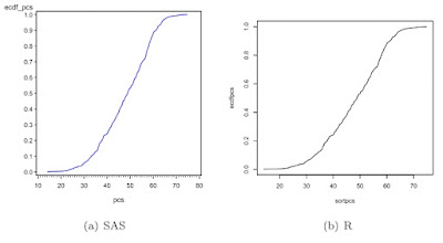
In SAS, we first read the data from a locally stored Stata data set. Then, we calculate the empirical CDF for pcs. We do this by first sorting (1.5.6) on pcs. Then the order statistic of the observation divided by the total number of obervations is the empirical probability that X ≤ x. We find the number of observations using the nobs data set option (A.6.1) and the observation number using the _n_ implied variable (1.4.15). Then we can plot the empirical CDF using proc gplot (section 5.1.1) to make a scatterplot and a symbol statement with the j interpolation (as in section 1.13.5) to connect the points.
proc import datafile="C:\book\help.dta"
   out=help dbms=dta;
run;

proc sort data=help;
   by pcs;
run;

data help_a;
set help nobs=totalobs;
   ecdf_pcs = _n_ / totalobs;
run;

symbol1 i=j v=none c=blue;
proc gplot data=help_a;
   plot ecdf_pcs * pcs;
run;
quit;
R
Now, R. First, make the ECDF values in a similar fashion to SAS, then make an empty frame (5.1.1), then fill the frame with lines connecting the calculated values (5.2.1).
library(foreign)
ds <- read.dta
  ("http://www.math.smith.edu/sasr/datasets/help.dta")
attach(ds)
sortpcs <- sort(pcs)
ecdfpcs <- (1:length(sortpcs))/length(sortpcs)
plot(sortpcs, ecdfpcs, type="n")
lines(sortpcs, ecdfpcs)

7 comments:
Is there a simple way to replace every value in ds with a corresponding value of the empirical distribution?
i.e.
ds #returns# 2 2 3 1 10 2
sort(ds) #returns# 1 2 2 2 3 10
ecdf #returns# 1/6 4/6 4/6 4/6 5/6 1
we want ecdfv #returns# 4/6 4/6 5/6 1/6 1 4/6
ohh cool.... figured out.... look:
ecdfv <- c(length(ds))
for(i in 1:length(ds)){ecdfv[i] <- length(ds[ds<=ds[i]&!is.na(ds)])/length(ds[!is.na(ds)])}
:DD
Pretty cool, Robert. I can imagine another solution where you'd attach an ID vector in the original order, compute the ECDF as we outline above, then re-sort on the ID vector to find the value of the ECDF in the original order (or save it in place, if that's the point). Here's my ugly version of that approach:
myvec <- c(2,2,3,1,10,2)
vecid <- 1:length(myvec)
mydata <- data.frame(cbind(myvec,vecid))
mydata <- mydata[order(myvec),]
mydata$myvec <- (1:length(mydata$myvec))/length(mydata$myvec)
mydata <- mydata[order(mydata$vecid),]
But looking this over, I see that it does not handle ties correctly.(Nor does our code in the example above.)
Can you explain how your code handles ties correctly? I can't see it.
Thanks!
Could we use the same method in case of a bivariate empirical cumulative density function ?
In SAS, Is there any one knows another than using the procedure KDE ? Thank you for your help .
Could we use the same method in case of a bivariate empirical cumulative density function ?
In SAS, Is there any one knows another than using the procedure KDE ? Thank you for your help .
What about the ecdf generated by stats::ecdf?
x<-ecdf(pcs)
plot(x,pch=NA)
Post a Comment