Example 7.12: Calculate and plot a running average

The Law of Large Numbers concerns the stability of the mean, as sample sizes increase. This is an important topic in mathematical statistics. The convergence (or lack thereof, for certain distributions) can easily be visualized in SAS and R (see also Horton, Qian and Brown, 2004).

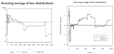
Assume that X1, X2, ..., Xn are independent and identically distributed realizations from some distribution with center mu. We define x-bar(k) as the average of the first k observations. Recall that because the expectation of a Cauchy random variable is undefined (Romano and Siegel, 1986) the sample average does not converge to the population parameter.

SAS
In SAS, we begin by writing a macro (section A.8) to generate the random variables and calculate the running average.

The macro runs a data step to generate the data and calculate the average after each value is generated using the sum function (section 1.8.1). The macro accepts the name of a data set to hold the variates and their running average, the number of random variates to generate, and the argument(s) to the rand function (section 1.10) so that variates from many distributions can be generated. For the purposes of making a dramatic example, we set a fixed random number seed (section 1.10.9).

%macro runave(outdata=, n=, distparms=) ;
data &outdata; 
call streaminit(1984);
do i = 1 to &n;
   x = rand &distparms;
   runtot = sum(x, runtot);
   avex = runtot/i;
   output;
  end;
run;
%mend runave;

In this example, we compare the Cauchy distribution to a t distribution with 4 degrees of freedom (for which the average does converge to the mean) for 1000 observations. To do this, we call the macro twice.

%runave(outdata=cauchy, n=1000, distparms= ("CAUCHY"));
%runave(outdata=t4, n=1000, distparms= ('T',4));

To plot the two running averages on a single figure, we combine the two data sets, using the in= data set option to identify which data set each observation came from. Then we plot the two curves using the a*b=c syntax for proc gplot (section 5.2.2). To connect the dots and choose line styles and colors, we use the symbol statement (sections 5.3.9-11), and a title statement (section 5.2.9) to add a title. SAS generates a legend by default with the a*b=c syntax.

data c_t4;
set cauchy t4 (in=t4);
if t4 then dist="t with 4 df";
  else dist="Cauchy";
run;

symbol1 i=j c=black l=1 w=2;
symbol2 i=j c=black l=2 w=2;

title"Running average of two distributions";
proc gplot data=c_t4;
   plot avex * i = dist / vref=0;
run;
quit;

R
Within R, we define a function (section B.5.2) to calculate the running average for a given vector, again allowing for variates from many distributions to be generated.

runave <- function(n, gendist, ...) {
   x <- gendist(n, ...)
   avex <- numeric(n)
   for (k in 1:n) {
      avex[k] <- mean(x[1:k])
   }
   return(data.frame(x, avex))
}

Next, we generate the data, using our new function. To make sure we have a nice example, we first set a fixed seed (section 1.10.9).

vals <- 1000
set.seed(1984)
cauchy <- runave(vals, rcauchy)
t4 <- runave(vals, rt, 4)

Finally, we're ready to plot. We begin by making an empty plot with the correct x and y limits, using the type="n" specification (section 5.1.1). We then plot the running average using the lines function (section 5.2.1) and varying the line style (section 5.3.9) and thickness (section 5.3.11) with the lty and lwd specification. Finally we add a title (section 5.2.9) and a legend (section 5.2.14).

plot(c(cauchy$avex, t4$avex), xlim=c(1, vals), type="n")
lines(1:vals, cauchy$avex, lty=1, lwd=2)
lines(1:vals, t4$avex, lty=2, lwd=2)
abline(0, 0)
title("Running average of two distributions")
legend(vals*.6, -1, legend=c("Cauchy", "t with 4 df"), 
   lwd=2, lty=c(1,2))