Example 7.30: Simulate censored survival data

To simulate survival data with censoring, we need to model the hazard functions for both time to event and time to censoring.

We simulate both event times from a Weibull distribution with a scale parameter of 1 (this is equivalent to an exponential random variable). The event time has a Weibull shape parameter of 0.002 times a linear predictor, while the censoring time has a Weibull shape parameter of 0.004. A scale of 1 implies a constant (exponential) baseline hazard, but this can be modified by specifying other scale parameters for the Weibull random variables.

First we'll simulate the data, then we'll fit a Cox proportional hazards regression model (section 4.3.1) to see the results.

Simulation is relatively straightforward, and is helpful in concretizing the notation often used in discussion survival data. After setting some parameters, we generate some covariate values, then simply draw an event time and a censoring time. The minimum of these is "observed" and we record whether it was the event time or the censoring time.

SAS

data simcox;
  beta1 = 2;
  beta2 = -1;
  lambdat = 0.002; *baseline hazard;
  lambdac = 0.004; *censoring hazard;
  do i = 1 to 10000;
    x1 = normal(0);
    x2 = normal(0);
    linpred = exp(-beta1*x1 - beta2*x2);
    t = rand("WEIBULL", 1, lambdaT * linpred);
    * time of event;
    c = rand("WEIBULL", 1, lambdaC);
           * time of censoring;
    time = min(t, c);    * which came first?;
    censored = (c lt t);
    output;
  end;
run;

The phreg procedure (section 4.3.1) will show us the effects of the censoring as well as the results of fitting the regression model. We use the ODS system to reduce the output.

ods select censoredsummary parameterestimates;
proc phreg data=simcox;
  model time*censored(1) = x1 x2;
run;

The PHREG Procedure

Summary of the Number of Event and Censored Values
 
                                     Percent
   Total       Event    Censored    Censored
   10000        5971        4029       40.29

          Analysis of Maximum Likelihood Estimates
 
                Parameter    Standard
Parameter  DF    Estimate       Error  Chi-Square  Pr > ChiSq

x1          1     1.98628     0.02213   8059.0716      <.0001
x2          1    -1.01310     0.01583   4098.0277      <.0001

Analysis of Maximum Likelihood Estimates
 
             Hazard
Parameter     Ratio

x1            7.288
x2            0.363

R

n = 10000
beta1 = 2; beta2 = -1
lambdaT = .002 # baseline hazard
lambdaC = .004  # hazard of censoring

x1 = rnorm(n,0)
x2 = rnorm(n,0)
# true event time
T = rweibull(n, shape=1, scale=lambdaT*exp(-beta1*x1-beta2*x2)) 
C = rweibull(n, shape=1, scale=lambdaC)   #censoring time
time = pmin(T,C)  #observed time is min of censored and true
event = time==T   # set to 1 if event is observed

Having generated the data, we assess the effects of censoring with the table() function (section 2.2.1) and load the survival() library to fit the Cox model.

> table(event)
event
FALSE  TRUE 
 4083  5917 

> library(survival)
> coxph(Surv(time, event)~ x1 + x2, method="breslow")
Call:
coxph(formula = Surv(time, event) ~ x1 + x2, method = "breslow")


    coef exp(coef) se(coef)     z p
x1  1.98     7.236   0.0222  89.2 0
x2 -1.02     0.359   0.0160 -64.2 0

Likelihood ratio test=11369  on 2 df, p=0  n= 10000 

These parameters result in data where approximately 40% of the observations are censored. The parameter estimates are similar to the true parameter values.

Example 7.29: Bubble plots colored by a fourth variable

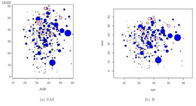
In Example 7.28, we generated a bubble plot showing the relationship among CESD, age, and number of drinks, for women. An anonymous commenter asked whether it would be possible to color the circles according to gender. In the comments, we showed simple code for this in R and hinted at a SAS solution for two colors. Here we show in detail what the SAS code would look like, and revisit the R code.


SAS

For SAS, we have to make two separate variables-- one with the CESD for the females, and another for the males. For the other gender, these gender-specific variables will have missing values. We'll do this using conditioning (section 1.11.2).

libname k "c:\book";

data twocolors;
set k.help;
  if female eq 1 then femalecesd = cesd;
  else malecesd = cesd;
run;

Now we can use the bubble2 statement (close kin of the plot2 statement, section 5.1.2) to add both gender-specific variables to the plot. While we're at it, we relabel the x-axis to no longer be gender specific and specify that the right y-axis is not to be labeled.

proc gplot data = twocolors;
bubble malecesd*age=i1 / bscale = radius bsize=200 
                           bcolor = blue bfill = solid;
bubble2 femalecesd*age=i1 / bscale = radius bsize = 200 
                           bcolor = pink bfill = solid noaxis;
label malecesd="CESD";
run;

As in the previous bubble plot example, the scale is manipulated arbitrarily so that the SAS and R figures are similar.

We're somewhat fortunate here that the range of the two gendered CESD scores are similar

R

In the comments for Example 7.28, we suggested the following simple R code.

load(url("http://www.math.smith.edu/sasr/datasets/savedfile"))
femalealc = subset(ds, female==1 & substance=="alcohol")
malealc = subset(ds, female==0 & substance=="alcohol")
with(malealc, symbols(age, cesd, circles=i1,
inches=1/5, bg="blue"))
with(femalealc, symbols(age, cesd, circles=i1,
inches=1/5, bg="pink", add=TRUE))

While this does generate a plot, it could be misleading, in that the scale of the circle sizes is relative to the largest value within each symbols() call. While this could be desirable, it's more likely that we'd like a single scale for the circles. R code for this can be made in a single statement:

load(url("http://www.math.smith.edu/sasr/datasets/savedfile"))
attach(ds)
symbols(age, cesd, circles=i1,inches=1/5, 
             bg=ifelse(female==1,"pink","blue")) 

Here the ifelse() function (section 1.11.2) generates a different circle fill color depending on the value of female.

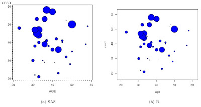
The resulting plots are shown below.

Example 7.28: Bubble plots

A bubble plot is a means of displaying 3 variables in a scatterplot. The z dimension is presented in the size of the plot symbol, typically a circle. The area or radius of the circle plotted is proportional to the value of the third variable. This can be a very effective data presentation method. For example, consider Andrew Gelman's recent re-presentation of health expenditure/survival data/annual number of doctor visits per person. On the other hand, Edward Tufte suggests that such representations are ambiguous, in that it is often unclear whether the area, radius, or height reflects the third variable. In addition, he reports that humans tend not to be good judges of relative area.

However, other means of presenting three dimensions on a flat screen or piece of paper often rely on visual cues regarding perspective, which some find difficult to judge.

Here we demonstrate SAS and R bubble plots using the HELP data set used in our book. We show a plot of depression by age, with bubble size proportional to the average number of drinks per day. To make the plot a little easier to read, we show this only for female alcohol abusers.

SAS

In SAS, we can use the bubble statement in proc gplot. We demonstrate here the use of the where data set option (section 1.5.1) for subsetting, which allows us to avoid using any data steps. SAS allows the circle area or radius to be proportional to the third variable; we choose the radius for compatibility with R. We alter the size of the circles for the same reason. We also demonstrate options for coloring in the filled circles.

libname k "c:\book";

proc gplot data = k.help (where=((female eq 1) 
                    and (substance eq "alcohol")));
bubble cesd*age=i1 / bscale = radius bsize=60 
                           bcolor=blue bfill=solid;
run;

R

In R, we can use the symbols() function for the plot. Here we also demonstrate reading in data previously saved in native R format (section 1.1.1), as well as the subset() function and the with() function (the latter appears in section 1.3.1). The inches option is an arbitrary scale factor. We note that the symbols() function has a great deal of additional capability-- it can substitute squares for circles for plotting the third variable, and add additional dimensions with rectangles or stars. Proportions can be displayed with thermometers, and boxplots can also be displayed.

load(url("http://www.math.smith.edu/sasr/datasets/savedfile"))
femalealc = subset(ds, female==1 & substance=="alcohol")
with(femalealc, symbols(age, cesd, circles=i1, 
                                 inches=1/5, bg="blue"))

The results are shown below. It appears that younger women with more depressive symptoms tend to report more drinking.

Example 7.27: probability question reconsidered

In Example 7.26, we considered a problem, from the xkcd blog:

Suppose I choose two (different) real numbers, by any process I choose. Then I select one at random (p= .5) to show Nick. Nick must guess whether the other is smaller or larger. Being right 50% of the time is easy. Can he do better?

Randall Munroe offers a solution which we tested in the previous example. However, his logic may not be obvious to all readers. Instead, Martin Kulldorff, author of the SaTScan software for cluster detection, offers the following intuition. Suppose Nick chooses a number k. If the first number is bigger than k, he'll guess that the hidden number is smaller, and vice versa. Let's condition to see what will happen. If both numbers are bigger than k, Nick will be right 50% of the time. If both are smaller than k, he'll also be right 50% of the time. But whenever the two numbers straddle k, he'll be right 100% of the time. So in the margin, he'll be right more than 50% of the time (because the two numbers are not identical). This strategy will sometimes work if I don't know Nick is using it and he makes a lucky choice of k. But even if I know Nick's strategy, he will still gain a rate over 50% by simply choosing k at random.

Munroe's strategy is the same as that outlined here, if we choose

k = log(u/(1-u))

where u is a Uniform(0,1) random variate, though this has a similar problem to Munroe's approach, in practice-- k rarely (only .000000002 of the time) exceeds about 20 in absolute value. A more effective strategy would be to choose k from a distribution with values more uniform across the reals. In the following code we use a Cauchy distribution (see section 1.10.1) spreading it out even further by multiplying each pseudo-random number by 1000.

SAS

The code is similar to that shown in the previous example, but does not require computing the function of the observed value.

data test2;
  do i = 1 to 100000;
    real1 = uniform(0) * 1000 + 1000;
    real2 = uniform(0) * 1000 + 1000;
 if uniform(0) gt .5 then do;
      env1 = real1;
   env2 = real2;
   end;
 else do;
   env1 = real2;
   env2 = real1;
   end;
 if (env1 gt (rand("CAUCHY") * 1000)) then guess = "l";
 else guess = "h";
 correct = (((env1 < env2) and (guess eq "h")) or 
              ((env1 > env2) and (guess eq "l"))) ;
 output;
 end;
run;

proc freq data = test2;
tables correct / binomial (level='1');
run;

The FREQ Procedure

                                    Cumulative    Cumulative
correct    Frequency     Percent     Frequency      Percent
------------------------------------------------------------
      0       48315       48.32         48315        48.32
      1       51685       51.69        100000       100.00


Proportion                0.5169
ASE                       0.0016
95% Lower Conf Limit      0.5138
95% Upper Conf Limit      0.5199

Exact Conf Limits
95% Lower Conf Limit      0.5137
95% Upper Conf Limit      0.5200

ASE under H0              0.0016
Z                        10.6569
One-sided Pr >  Z         <.0001
Two-sided Pr > |Z|        <.0001

Sample Size = 100000

R

mk1 = function(n) {
   real1 = runif(n) * 1000 + 1000
   real2 = runif(n) * 1000 + 1000
   pickenv = (runif(n) < .5)
   env1 = ifelse(pickenv,real1,real2)
   env2 = ifelse(!pickenv,real1,real2)
   k = rcauchy(n) * 1000
   guess = ifelse(env1 > k,"lower","higher")
   correct = ((env1 < env2) & (guess == "higher"))  | ((env1 > env2) &
      (guess == "lower"))
   return(correct)
}

> binom.test(sum(mk1(100000)),100000)

        Exact binomial test

data:  sum(mk1(1e+05)) and 1e+05 
number of successes = 51764, number of trials = 1e+05, p-value <
2.2e-16
alternative hypothesis: true probability of success is not equal to 0.5 
95 percent confidence interval:
 0.5145375 0.5207415 
sample estimates:
probability of success 
               0.51764 

This approach is so much better than the other that we can detect the effect in only 100,000 trials!

Example 7.26: probability question

Here's a surprising problem, from the xkcd blog.

Suppose I choose two (different) real numbers, by any process I choose. Then I select one at random (p= .5) to show Nick. Nick must guess whether the other is smaller or larger. Being right 50% of the time is easy. Can he do better?

Of course, it wouldn't be an interesting question if the answer was no. Randall Munroe (author of the xkcd webcomic) offers a solution as follows:

1. Call the number you see x.  
      Calculate p(x) = (e^x)/(1 + e^x)
2. Draw u, a random uniform(0,1).
3. If u < p(x) then guess the hidden number is 
      smaller than the revealed one.  Otherwise,
      guess that it is smaller.

Munroe shows that the probability of guessing correctly is

N = 0.5 * (1-p(A)) + 0.5 * p(B)

where A is the smaller of the two numbers. In practice, this only gains us an advantage when the observed value is between about -20 and 20-- outside that range, calculation of p(x) results in numbers so close to 0 or 1 that no improvement over a 50% rate can be achieved. If I knew Nick were using this method, I could keep him to a 50% rate by always choosing numbers over 1000 or so. He can improve Munroe's solution by using p(x/100000), though at the cost of a poorer improvement near 0.

We'll check the logic by simulating the experiment.

SAS

The SAS solution requires a lot of looping (section 1.11.1) and conditional execution (section 1.11.2).

data test;
  do i = 1 to 10000000;
    real1 = uniform(0) * 1000 + 1000;
    real2 = uniform(0) * 1000 + 1000;
 if uniform(0) gt .5 then do;
      env1 = real1;
   env2 = real2;
   end;
 else do;
   env1 = real2;
   env2 = real1;
   end;
 if uniform(0) lt (1/(1 + exp(-1 * env1/100000))) then guess = "l";
 else guess = "h";
 correct = ((env1 < env2) and (guess eq "h")) or 
              ((env1 > env2) and (guess eq "l")) ;
 output;
 end;
run;

We can test the performance using proc freq with the binomial option (section 2.1.9).

proc freq data = test;
tables correct / binomial;
run;

The FREQ Procedure

                                    Cumulative    Cumulative
correct    Frequency     Percent     Frequency      Percent
------------------------------------------------------------
      0     4996889       49.97       4996889        49.97
      1     5003111       50.03      10000000       100.00


Proportion                0.5003
ASE                       0.0002
95% Lower Conf Limit      0.5000
95% Upper Conf Limit      0.5006

Exact Conf Limits
95% Lower Conf Limit      0.5000
95% Upper Conf Limit      0.5006

ASE under H0              0.0002
Z                         1.9676
One-sided Pr >  Z         0.0246
Two-sided Pr > |Z|        0.0491

Sample Size = 10000000

We can just barely detect the improvement-- but it took 10,000,000 trials to find CI that reliably exclude the possibility of a 50% success rate.




R

We begin by writing a function to calculate p(x/100000).

xkcdprob = function(x) {
1/(1 + exp(-1 * x/100000))}

Then we write a function to perform the experiment n times. Here we use the same process for picking the two numbers, choosing them to be Uniform between 1000 and 2000. In the code below we use the ifelse() function (section 1.11.2) to decide which envelope is shown first. The vectorization in R allows us to avoid loops entirely in writing the code.

larger1 = function(n) {
real1 = runif(n) * 1000 + 1000
real2 = runif(n) * 1000 + 1000
pickenv = (runif(n) < .5)
env1 = ifelse(pickenv,real1,real2)
env2 = ifelse(!pickenv,real1,real2)
guess = ifelse(runif(n) < xkcdprob(env1),"lower","higher")
correct =  ((env1 < env2) & (guess == "higher"))  | ((env1 > env2) &
   (guess == "lower"))
return(correct)
}

Then we can run the experiment and check its results in one nested call, using the binom.test() function (section 2.1.9) to see whether the observed proportion is different from 0.5.

> binom.test(sum(larger1(10000000)),10000000)

        Exact binomial test

data:  sum(larger1(1e+07)) and 1e+07 
number of successes = 5003996, number of trials = 1e+07, p-value =
0.01150
alternative hypothesis: true probability of success is not equal to 0.5 
95 percent confidence interval:
 0.5000897 0.5007095 
sample estimates:
probability of success 
             0.5003996 

Example 7.25: compare draws with distribution

In example 7.24, we demonstrated a Metropolis-Hastings algorithm for generating observations from awkward distributions. In such settings it is desirable to assess the quality of draws by comparing them with the target distribution.

Recall that the distribution function is

f(y) = c e^(-y^4)(1+|y|)^3

The constant c was not needed to generate draws, but is required for calculation of the probability density function. We can find the normalizing constant c using symbolic mathematics software (try running it yourself using Wolfram Alpha). This yields a result .25 + (.75 * Pi^(.5) + Gamma(5/4) + Gamma(7/4) for the integral over the positive real line, which when doubled gives a value of c=6.809610784.



SAS

To compare the distribution of the variates with the truth, we first generate a density estimate using proc kde (sections 2.6.4, 5.1.16), saving the density estimates in a new data set.

ods select none;
proc kde data=mh;
  univar x / out=mhepdf;
run;
ods exclude none;

Then we generate the true values, using the constant calculated above.

data mh2;
  set mhepdf;
  true = 6.809610784**(-1) *
    exp(-value**4) * (1 + abs(value))**3;
run;

Finally, we can plot the estimated and true values together. We use the legend statement (section 5.2.14) to approximate the R legend created below.

legend1 position=(bottom center inside)
  across=1 noframe label=none value=(h=1.5);
axis1 label=(angle=90 "Density");
symbol1 i=j l=1 w=3 c=black;
symbol2 i=j l=2 w=3 c=black;
proc gplot data = mh2;
  plot (density true)*value / overlay vaxis = axis1 legend=legend1;
  label value="x" density="Simulated" true="True";
run;

R

In R, we begin by defining a function to calculate f(y)

pdfeval = function(x) {
   return(1/6.809610784*exp(-x^4)*(1+abs(x))^3)
}

The curve() function in R is useful for plotting values of functions over a range. We use it here to plot f(y). Then we use the density() function (section 5.1.16) to estimate the density function from the variates. Rather than save this information in an object, we use it as input to the lines function (section 5.2.1).

curve(pdfeval, from=-2, to=2, lwd=2, lty=2, type="l", 
   ylab="probability", xlab="Y")
lines(density(res), lwd=2, lty=1)
legend(-1, .1, legend=c("True", "Simulated"), 
   lty=2:1, lwd=2, cex=1.8, bty="n")

Results from both systems are plotted below.




We note that in each plot, the sampled variates appear to miss the distribution function near 0. This is an artifact of the default smoothing used by the density estimators, and could be tuned away.

Augmented support for complex survey designs in R

We'll get back to code examples later this week, but wanted to let you know about an R package with updated functionality in the meantime.

The appropriate analysis of sample surveys requires incorporation of complex design features, including stratification, clustering, weights, and finite population correction. These can be address in SAS and R for many common models. Section 6.8 of the book provides an overview of these methods.

Improved support for these designs in R is now available in the survey package. This includes support for multivariate analysis (factor analysis [section 6.7.2] and principal components), parallel processing on multicore computers, and access to database-backed design objects (which are particularly useful for large datasets).

In addition to the updates, package author Thomas Lumley has made the table of contents and preface available for his forthcoming book. Other helpful resources include Alan Zaslavsky's summary of survey analysis software.

Example 7.24: Sampling from a pathological distribution

Evans and Rosenthal consider ways to sample from a distribution with density given by:

f(y) = c e^(-y^4)(1+|y|)^3

where c is a normalizing constant and y is defined on the whole real line.

Use of the probability integral transform (section 1.10.8) is not feasible in this setting, given the complexity of inverting the cumulative density function.

The Metropolis--Hastings algorithm is a Markov Chain Monte Carlo (MCMC) method for obtaining samples from a probability distribution. The intuition behind this algorithm is that it chooses proposal probabilities so that after the process has converged we are generating draws from the desired distribution. A further discussion can be found on page 610 of Section 11.3 of the Evans and Rosenthal text, or on page 25 of Gelman et al.

We find the acceptance probability a(x, y) in terms of two densities, f(y) and q(x,y) (a proposal density, in our example, normal with specified mean and unit variance) so that

a(x,y) = min(1, [c*f(y)*q(y,x)]/[c*f(x)*q(x,y)]
       = min(1, [e^(-y^4+x^4)(1+|y|)^3]/[(1+|x|)^3]

where we omit some algebra.

Begin by picking an arbitrary value for X_1. The Metropolis--Hastings algorithm then proceeds by computing the value X_{n+1} as follows:

1. Generate y from a Normal(X_n, 1).
2. Compute a(x, y) as above.
3. With probability a(x, y), let X_{n+1} = y 
                             (i.e., use proposal value). 
   Otherwise, with probability 1-a(x, y), let X_{n+1} = X_n 
                             (i.e., keep previous value). 

The code allows for a burn-in period, which we set at 50,000 iterations, and a desired sample from the target distribution, which we make 5,000. To reduce auto-correlation, we take only every twentieth variate. In a later entry, we'll compare the resulting variates with the true distribution.

SAS

The SAS code is fairly straightforward.

data mh;
  burnin = 50000;  numvals = 5000; thin = 20;
  x = normal(0);
  do i = 1 to (burnin + (numvals * thin));
    y = normal(0) + x;
    switchprob = min(1, exp(-y**4 + x**4) *
     (1 + abs(y))**3 * (1 + abs(x))**(-3));
    if uniform(0) lt switchprob then x = y;
      * if we don't change x, the previous value is kept-- 
           no code needed;
    if (i gt burnin) and mod(i-burnin, thin) = 0 then output;
      * only start saving if we're past the burn-n period, 
           then thin out;
  end;
run;

R

In R we first define a function to compute a(x,y):

alphafun = function(x, y) { 
   return(exp(-y^4+x^4)*(1+abs(y))^3*
      (1+abs(x))^-3) 
} 

Then we proceed as in the SAS example.

numvals = 5000; burnin = 50000; thin = 20
res = numeric(numvals)
i = 1 
xn = rnorm(1) # arbitrary value to start
for (i in 1:(burnin + numvals * thin)) {
   propy = rnorm(1, xn, 1) 
   alpha = min(1, alphafun(xn, propy)) 
   xn = sample(c(propy, xn), 1, prob=c(alpha,1-alpha))
   if ((i > burnin) & ((i-burnin) %% thin == 0)) 
      res[(i-burnin)/thin] = xn 
} 

The resulting draws from the distribution are available in the res vector.