This is a topic that has come up with increasing frequency in grant proposals and article submissions. We'll begin by showing how to simulate data with the interaction, and in our next post we'll show how to assess power to detect the interaction using simulation.
As in our earlier post, our method is to construct the linear predictor and the link function separately. This should help to clarify the roles of the parameter values and the simulated data.
SAS
In keeping with Annisa Mike's question, we'll simulate the interaction between a categorical and a continuous covariate. We'll make the categorical covariate dichotomous and the continuous one normal. To keep things simple, we'll leave the main effects null-- that is, the effect of the continuous covariate when the dichotomous one is 0 is also 0.
data test;
do i = 1 to 1000;
    c = (i gt 500);
    x = normal(0);
    lp = -3 + 2*c*x;
    link_lp = exp(lp)/(1 + exp(lp));
    y = (uniform(0) lt link_lp);
 output;
end;
run;
In proc logistic, unlike other many other procedures, the default parameterization for categorical predictors is effect cell coding. This can lead to unexpected and confusing results. To get reference cell coding, use the syntax for the class statement shown below. This is similar to the default result for the glm procedure. If you need identical behavior to the glm procedure, use param = glm. The desc option re-orders the categories to use the smallest value as the reference category.
proc logistic data = test plots(only)=effect(clband);
class c (param = ref desc);
model y(event='1') = x|c;
run;
The plots(only)=effect(clband) construction in the proc logistic statement generates the plot shown above. If c=0, the probability y=1 is small for any value of x, and a slope of 0 for x is tenable. If c=1, the probability y=1 increases as x increases and nears 1 for large values of x.
The parameters estimated from the data show good fidelity to the selected values, though this is merely good fortune-- we'd expect the estimates to often be more different than this.
                              Standard         Wald
Parameter     DF   Estimate      Error   Chi-Square   Pr > ChiSq

Intercept      1    -3.0258     0.2168     194.7353       <.0001
x              1    -0.2618     0.2106       1.5459       0.2137
c         1    1    -0.0134     0.3387       0.0016       0.9685
x*c       1    1     2.0328     0.3168      41.1850       <.0001
R
As sometimes occurs, the R code resembles the SAS code. Creating the data, in fact, is quite similar. The main differences are in the names of the functions that generate the randomness and the vectorized syntax that avoids the looping of the SAS datastep.
c = rep(0:1,each=500)
x = rnorm(1000)
lp = -3 + 2*c*x
link_lp = exp(lp)/(1 + exp(lp))
y = (runif(1000) < link_lp)
We fit the logistic regression with the glm() function, and examine the parameter estimates.
log.int = glm(y~as.factor(c)*x, family=binomial)
summary(log.int)
Here, the estimate for the interaction term is further from the selected value than we lucked into with the SAS simulation, but the truth is well within any reasonable confidence limit.
                Estimate Std. Error z value Pr(>|z|)
(Intercept)      -3.3057     0.2443 -13.530  < 2e-16 ***
as.factor(c)1     0.4102     0.3502   1.171    0.241
x                 0.2259     0.2560   0.883    0.377
as.factor(c)1:x   1.7339     0.3507   4.944 7.66e-07 ***
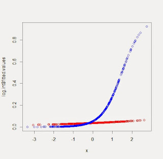
A simple plot of the predicted values can be made fairly easily. The predicted probabilities of y=1 reside in the summary object as log.int$fitted.values. We can color them according to the values of the categorical predictor by defining a color vector and then choosing a value from the vector for each observation. The resulting plot is shown below. If we wanted confidence bands as in the SAS example, we could get standard error for the (logit scale) predicted values using the predict() function with the se.fit option.
mycols = c("red","blue")
plot(log.int$fitted.values ~ x, col=mycols[c+1])
An unrelated note about aggregators: We love aggregators! Aggregators collect blogs that have similar coverage for the convenience of readers, and for blog authors they offer a way to reach new audiences. SAS and R is aggregated by R-bloggers, PROC-X, and statsblogs with our permission, and by at least 2 other aggregating services which have never contacted us. If you read this on an aggregator that does not credit the blogs it incorporates, please come visit us at SAS and R. We answer comments there and offer direct subscriptions if you like our content. In addition, no one is allowed to profit by this work under our license; if you see advertisements on this page, the aggregator is violating the terms by which we publish our work.


In the SAS example, you might want to use the CLPARM=wald option on the model statement. That produces a table that shows that the CI for the c and x parameters include zero, but the CIs for the Intercept and interaction terms do not.
ReplyDeleteHi!
ReplyDeleteThank you very much for your program.
Is it possible to use it when model consists of several binary variables Yes/No without contentious variable?
I tried to modify the code without success.